1 EvoLaps imports only one scenario at a time, but during the analysis, it is possible to save views of the imported scenario. For example, saving a clustering adds a scenario to the list of scenarios

2 ‘Play’ function has two modes: a normal mode (default) and an optional slice mode. In normal mode, the brush remains in the same position, but its width increases over time. In slice mode, the brush moves over time (translation), but its width remains constant. This width is adjustable as a percentage of the total phylogenetic tree duration (here 10%). Both modes include controls for pausing/resuming the animation and stopping it entirely. During a pause, graphical parameters of the scenario (HPD display, path colors, gradients, etc.) can be adjusted on the fly. Both modes respect the selected animation speed, controlled by parameter ‘v’ ranging from 0.1 (slowest) to 0.9 (fastest).

3 A default brush is displayed at the center of the phylohgenetic tree display and the phylogeographic scenario is restricted to this selection The size and position of the selection brush are variable, either determined by the user on-the-fly or automatically (Play mode) The use of a selection brush enables the display of a phylogeographic scenario limited to a specific clade and/or time slice, with paths that may be partial (see 'partial paths' below).

4 Highlighting and cross-selection between the phylogeographic scenario and the phylogenetic tree. Pointing to a node in the tree highlights its origin all the way to the root, as well as the underlying clade, using two user-selected colors: an ‘upstream’ color and a ‘downstream’ color, respectively. This process automatically reflects on the phylogeographic scenario: the ‘upstream’ color overlays the phylogeographic scenario from its starting point to the selected node, while the associated migration paths of the clade are highlighted with the ‘downstream’ color. Conversely, pointing to a path in the phylogeographic scenario allows highlighting the upstream and downstream areas of the phylogeographic scenario, as well as the corresponding branches within the phylogenetic tree. Selection is performed using the same method, but with a mouse click, allowing the user to preserve the highlighted areas. The ‘upstream’ and ‘downstream’ colors can vary (user’s settings) between different selections.

5 Partials paths

• the path between two points is ‘complete’ when the corresponding nodes within the phylogenetic tree are within the brush selection
• the path is ‘total partial’ if none of the associated nodes are within the brush selection, which lies between the two nodes (father vs son) of the tree
• if the parent node is within the selection but not the child node, the path is ‘downstream partial’
• if the child node is within the selection but not the parent node, the path is ‘upstream partial’

6 Camera waypoints allow you to create smooth, animated transitions—ideal for producing animations to include as supplementary material in a publication.

• navigate through the scenario by adjusting latitude/longitude, altitude (zoom), pitch and bearing, add as many waypoints as needed.
• set the transition time between waypoints by clicking .
• set the pause duration at each waypoint by clicking .
• click the play button to preview the animation, and record it using screen capture software.

7 Library ...

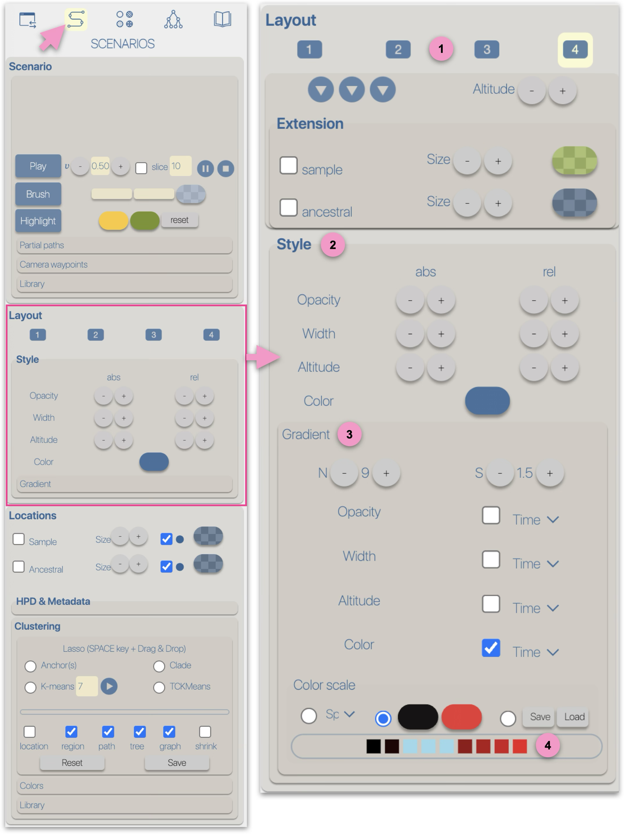
1 The graphical representations of phylogeographic scenarios (layouts) are grouped into families (currently four), based on the methods used to compute a path connecting points (latitude/longitude) associated with nodes of the phylogenetic tree (a parent node to its child nodes).

For example, and without going into too much technical detail, layout family 1 implements a Bézier curve smoothing technique using three control points:

• a first point (latitude/longitude) associated with a parent node,
• a second point (latitude/longitude) associated with a child node,
• an intermediate point calculated as the average of the latitude and longitude of the two previous points.

Layout family 2 also uses a smoothing method based on 3 control points: the points associated with the parent and child nodes, but the intermediate point lies on a circle of radius *r* and at an angle *alpha*, with the circle centered on the average latitude and longitude of the parent/child points.

Layout family 3 uses a smoothing method based on 4 control points: the points associated with the parent and child nodes, and two intermediate points, each located on a circle of radius *r* and angle *alpha*, centered respectively on the parent and the child node.

Due to these different computation methods, each layout family is associated with specific parameters/controls. For example, family 1 provides an offset control for the latitude and longitude of the intermediate point. Family 2 offers offset controls for the radius and angle of the circle carrying the intermediate point.

Other layout-family-specific parameters allow for visual variations of the phylogeographic scenarios. For instance, family 4, which introduces a notion of altitude, provides variants based on the path shape: linear, curved, or rectangular, as well as an altitude offset and the drawing of the vertical projection of the points onto the surface.

Nota Bene: the graphical rendering quality of phylogeographic scenarios varies depending on the different families/methods used to compute the paths, and may be more or less suitable depending on the nature of the dataset. It is recommended to test them.

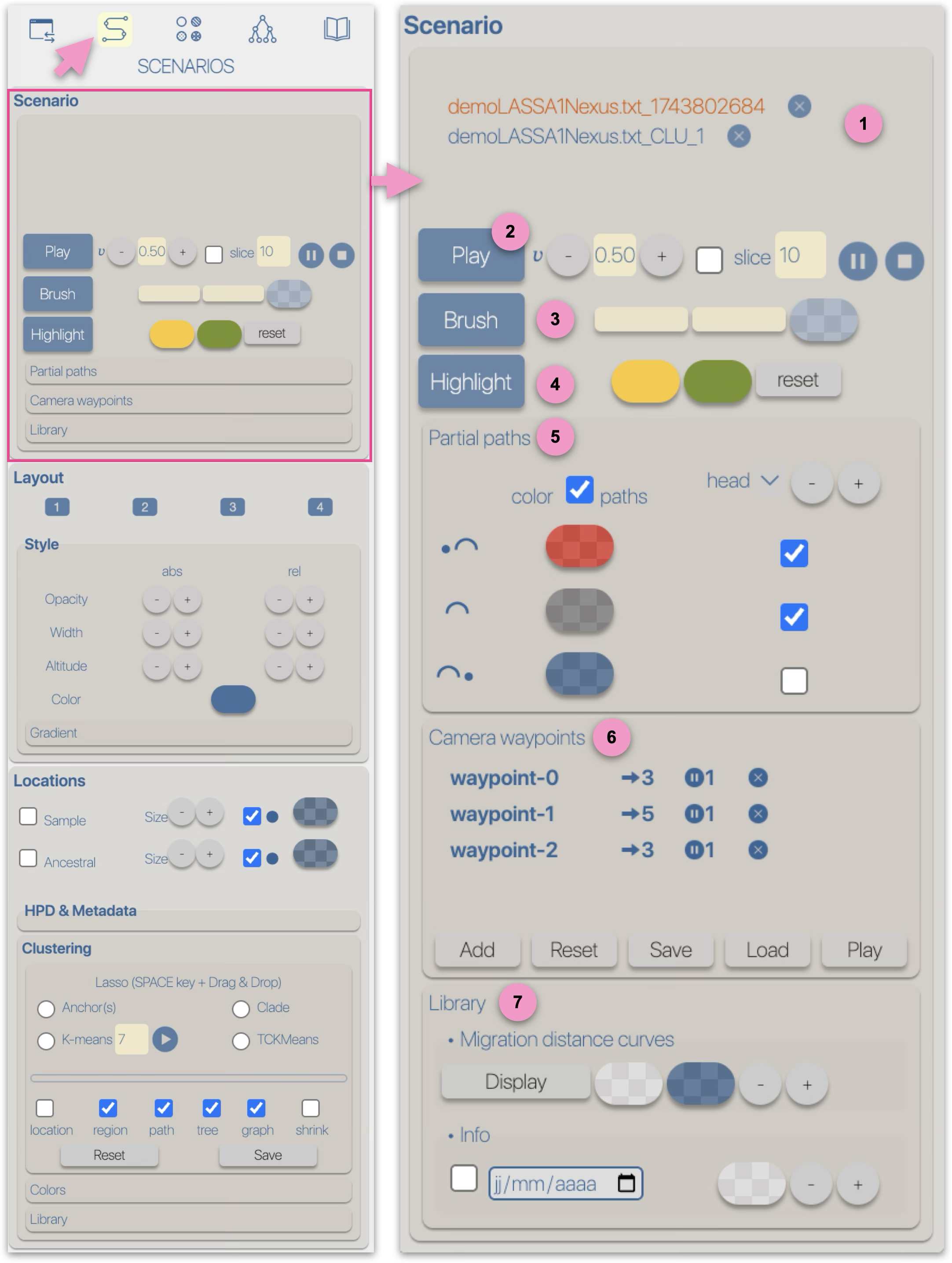
2 Regardless of the layout used to represent the phylogeographic scenario, it can be modified using four graphical variables: opacity, stroke thickness, altitude (curvature), and color. Apart from color, modifications (increase/decrease) can be either 'absolute' (abs): the same value is applied to all paths in the scenario, or relative (rel): the existing value of each path is incremented (or decremented) individually. These modifications can be performed manually (using -/+ buttons) or automatically by applying a gradient.

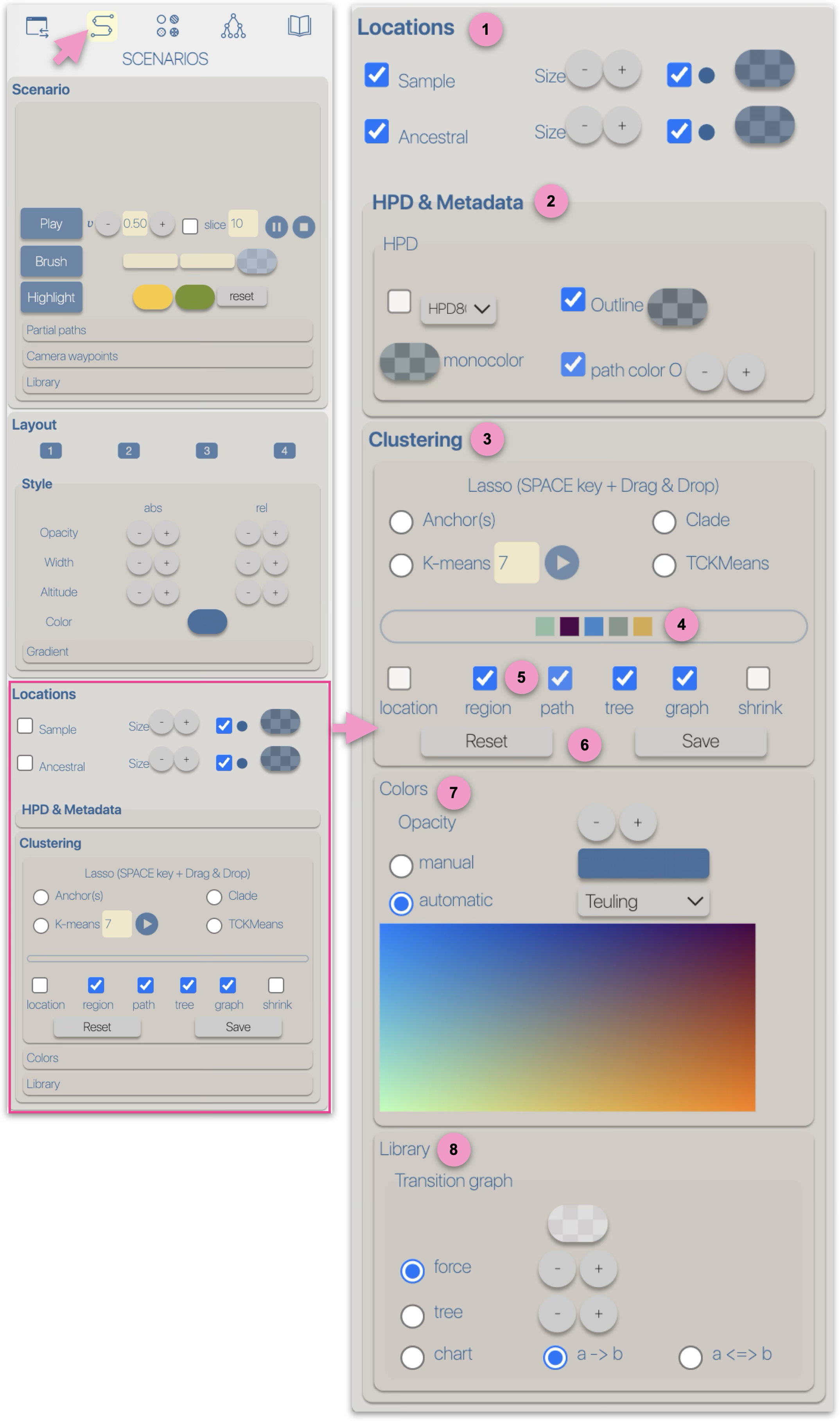
3 Gradient Opacity, stroke thickness, altitude (curvature), and color can be associated with a gradient. This gradient is configurable:

• N is the number of classes
• S is a stringency parameter between classes — the higher the S value, the stronger the contrast between classes

• Time: this gradient is based on the cumulative branch length from the node to the root of the phylogenetic tree
• Distance: this gradient is computed as the sum of geographical distances along the path from the node to the tree root (bottom-up recursive process). It is the sum of orthodromic distances (e.g., great-circle distances based on latitude and longitude between two points on a sphere)
• Speed: this gradient is based on the Distance/Time ratio of the two previous gradients

• using a color scale. The colors in a scale are optimized, and the choice of scales is restricted depending on the number of gradient classes
• selecting a start and end color
• saving/loading a list of specific colors. The colors must be in hexadecimal format without transparency, listed in square brackets, for example: ["#d53e4f", "#fc8d59", "#fee08b", "#b5e61d", "#22b14b", "#a349a4", "#3288bd"]. In this example, the gradient can use up to 7 classes. The colors will be used in the order they appear in the list.

4 The color gradient classes (associated with time, distance, or speed) are represented by a list of colored boxes. Clicking on a box allows you to change the color of the corresponding class. Assigning the same color to multiple adjacent classes enables a non-linear color gradient.

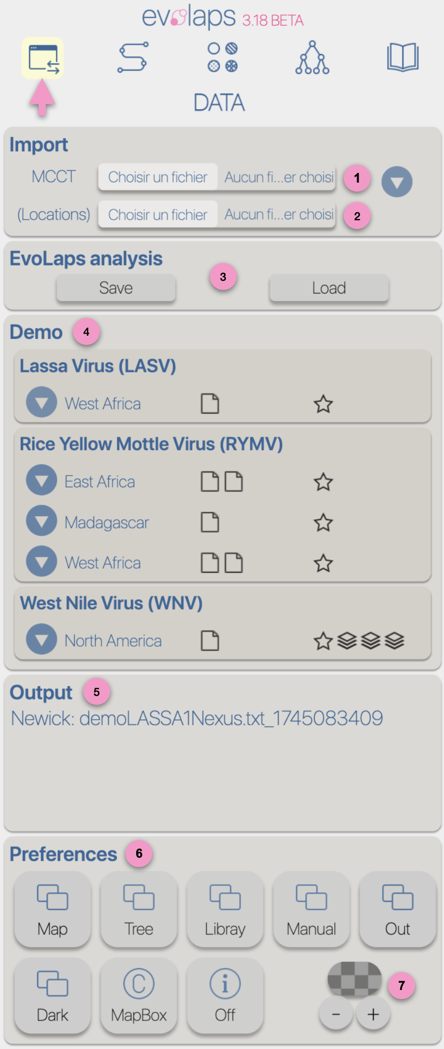
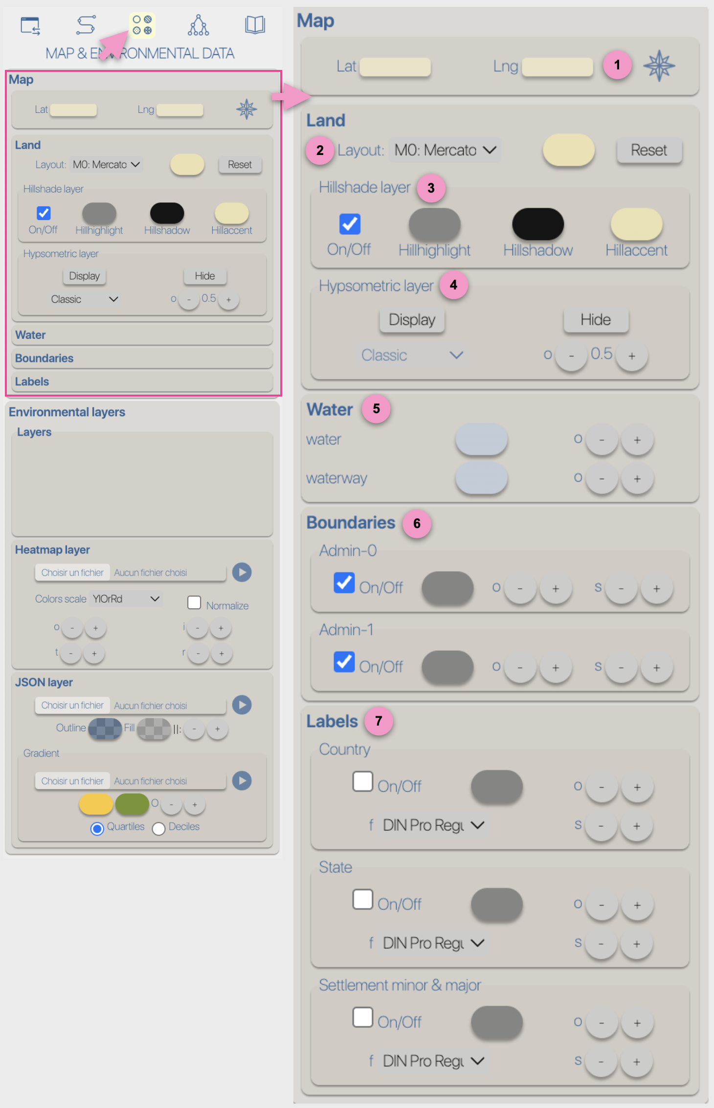
1 Display or hide ancestral and sampled locations with customizable color and transparency settings, using filled or outlined circles with variable sizes.

2 Display or hide HPDs for a selected percentage with customizable color and transparency settings, using filled and/or outlined areas. These areas can share the same color or inherit the color of their corresponding path.

3 EvoLaps incorporates a set of tools to group ancestral and sampled localities into spatial clusters of varying sizes. A clustering operation can be used not only to simplify the scenario but also to color it. This allows users to define zones and visualize associated incoming/outgoing paths (receiver/emitter zones).

Nota Bene: during clustering, all ancestral and sampled locations do not necessarily have to belong to a cluster. For example, it is possible to define a single cluster using the Lasso tool simply to better visualize the corresponding incoming/outgoing paths.

• Lasso clustering: to define a cluster using the Lasso tool, hold down the space key, then click on the map and draw a region that includes the locations (ancestral and sampled) you want to include in the cluster. The Lasso can be used to split or merge existing clusters — for example, to refine a previous clustering based on the 'KMeans' method. The cluster color can be selected manually or automatically (see below). The Lasso is a simple, dynamic, and fast method to visualize the incoming and outgoing paths of a given geographic area.
• Anchor clustering: clicking on the geographic map triggers the display of an anchor at the coordinates pointed to. Anchors serve as potential clusters and are movable (drag & drop) or removable (right-clicked). The nearest localities to the anchor (measured by Euclidean distances) are colored with the anchor’s hue, indicating their cluster membership. Therefore, the user can move the desired number of dynamic anchors/clusters on the geographic map. Clusters are then represented as minimum convex hull polygons, with fill color specified by their original anchor. The anchor color can be selected manually or automatically (see below).
• The Kmeans algorithm requires an initial number of seeds (k, cluster centroids) randomly generated within the boundaries of locations. Then, iteratively until no change, locations are assigned to their closest centroid based on the Euclidean distance, and centroids are updated. This algorithm can be used as a heuristic to automatically define geographically consistent groups, which can be adjusted by the user afterwards.
• New clustering methods will soon be available.

4 This panel displays the list of current clusters. Each cluster is represented by a colored box matching its assigned color. A left-click on a box allows you either to delete the cluster or to change its color.

5 List of operations available when a list of clusters is defined:

• Location: color ancestral and sampled locations using the color of their corresponding cluster
• Region: define cluster areas (minimum convex hull polygons)
• Path: color outgoing paths from each cluster with the color of the origin cluster
• Tree: color the phylogenetic tree
• Graph: compute and display the inter-cluster transition graph (see below)
• Shrink: simplify the phylogeographic scenario by replacing the latitude/longitude of ancestral and sampled locations with the latitude/longitude of their cluster centroid

6

• Reset: reset the cluster list
• Save: save the current cluster list as a new phylogeographic scenario (see the scenario list)

7 Cluster colors can be selected manually or automatically. The automatic mode is based on a 2D color matrix, according to the latitude and longitude of the centroid of the cluster (Lasso, KMeans) or the latitude/longitude of an anchor when it is created (Anchor). The opacity is the same for all clusters and can vary from 0.1 to 1.

8 Assigning localities to spatial clusters yields an inter-cluster transition graph. EvoLaps currently proposes 3 types of transition graph: a forcefield graph, a tree graph, and a matrix exchange graph (chart). For more information on transition graphs, see the associated section.

1 This box displays the latitude and longitude coordinates of the mouse pointer on the map. The compass rose icon allows the display of the latitude/longitude of the current field of view.

2 Map background Currently, EvoLaps offers an editable 'Alpha' map and a satellite map with or without labels. The color picker next to the map menu allows you to choose a terrain color. The 'reset' button restores the default map settings.

3 Hillshade layer This section is dedicated to terrain shading: show or hide, with customizable Hillhighlight, Hillshadow, and Hillaccent colors. For example, to create a softer terrain appearance, replace the default black Hillshadow color with a lighter one.

4 Hypsometric layer Map coloring by altitude class. The 'Display' button triggers the computation and display of the Hypsometric layer. This calculation may take several seconds depending on the size of the geographic map. It is recommended to zoom out the scenario display area and set pitch and bearing to zero before enabling it. This layer can be displayed using several color palettes and with adjustable opacity.

5 Hydrometric layers Color and opacity settings for hydrometric layers. These are the map’s default layers; see below for how to add custom hydrometric layers, for instance to ensure visibility even when significantly zoomed out (environmental data).

6 Border settings Display, color, opacity, and size settings for borders.

7 Map annotations Display settings for labels (country, administrative regions, localities): including color, opacity, and font.

1 List of environmental layers. The left checkbox allows you to display or hide the layer. The right radiobutton allows you to select and modify the layer (colors, opacity, etc.).

2Heatmap layers can be used to visualize spatial distribution of data. The heatmap layer internally implements Gaussian Kernel Density Estimation to render heatmaps. the data format is as follows:

• Colors scaleThe color palette used in the heatmap
• o (opacity) Opacity of the heatmap
• i (intensity) Value that is multiplied with the total weight at a pixel to obtain the final weight. A value larger than 1 biases the output color towards the higher end of the spectrum, and a value less than 1 biases the output color towards the lower end of the spectrum.
• t (threshold)The HeatmapLayer reduces the opacity of the pixels with relatively low weight to create a fading effect at the edge. A larger threshold smoothens the boundaries of color blobs, while making pixels with low relative weight harder to spot (due to low alpha value).
• r (radius)Radius of the circle in pixels, to which the weight of an object is distributed.

3JSON layers The GeoJsonLayer renders GeoJSON formatted data as polygons, lines and points (circles, icons and/or texts)