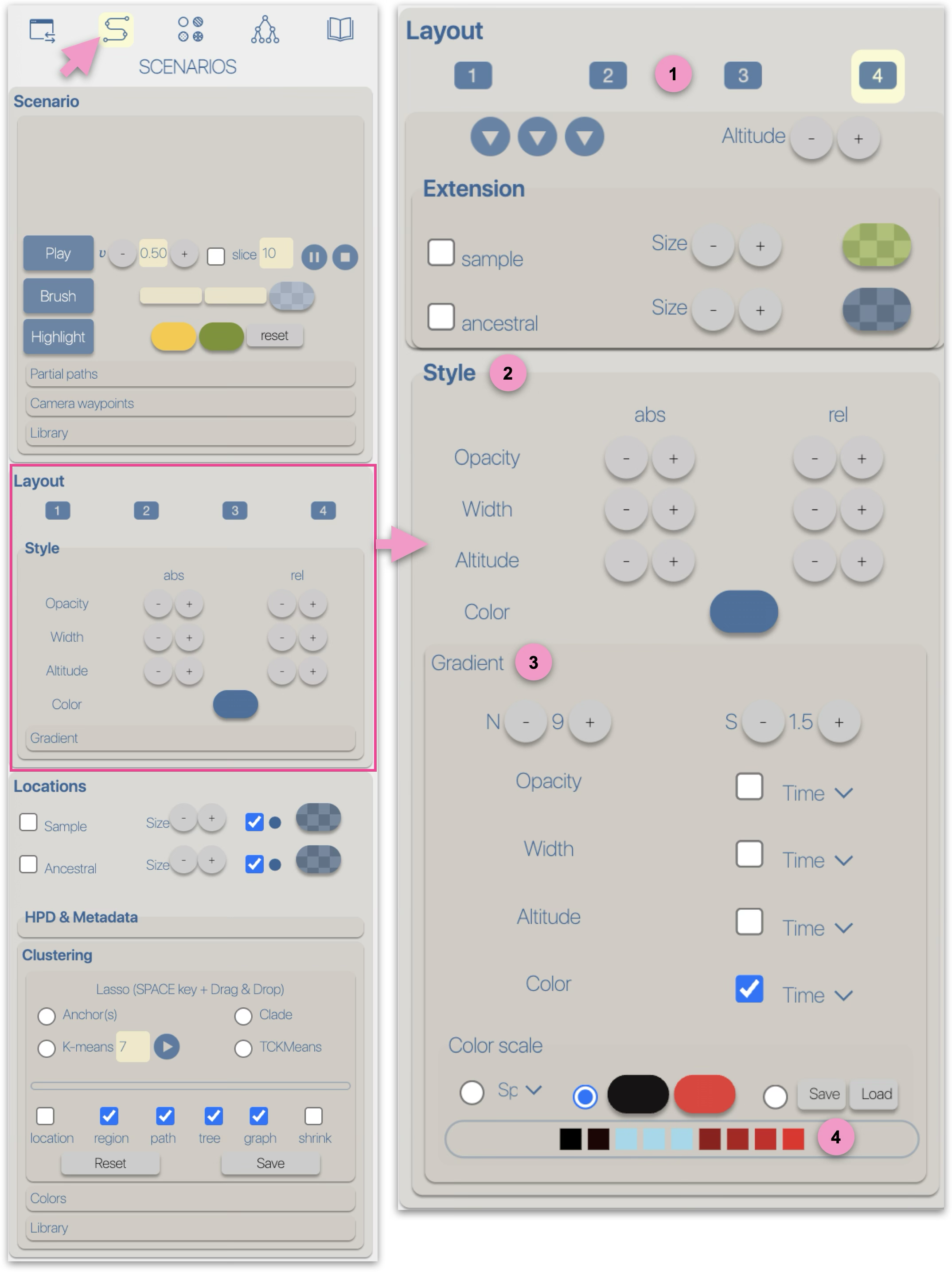
1 The graphical representations of phylogeographic scenarios (layouts) are grouped into families (currently four), based on the methods used to compute a path connecting points (latitude/longitude) associated with nodes of the phylogenetic tree (a parent node to its child nodes). For example, and without going into too much technical detail, layout family 1 implements a Bézier curve smoothing technique using three control points:

• a first point (latitude/longitude) associated with a parent node,
• a second point (latitude/longitude) associated with a child node,
• an intermediate point calculated as the average of the latitude and longitude of the two previous points.

Layout family 2 also uses a smoothing method based on 3 control points: the points associated with the parent and child nodes, but the intermediate point lies on a circle of radius *r* and at an angle *alpha*, with the circle centered on the average latitude and longitude of the parent/child points.

Layout family 3 uses a smoothing method based on 4 control points: the points associated with the parent and child nodes, and two intermediate points, each located on a circle of radius *r* and angle *alpha*, centered respectively on the parent and the child node.

Due to these different computation methods, each layout family is associated with specific parameters/controls. For example, family 1 provides an offset control for the latitude and longitude of the intermediate point. Family 2 offers offset controls for the radius and angle of the circle carrying the intermediate point.

Other layout-family-specific parameters allow for visual variations of the phylogeographic scenarios. For instance, family 4, which introduces a notion of altitude, provides variants based on the path shape: linear, curved, or rectangular, as well as an altitude offset and the drawing of the vertical projection of the points onto the surface.

Nota Bene: the graphical rendering quality of a phylogeographic scenario varies depending on the different families/methods used to compute the paths, and may be more or less suitable depending on the nature of the dataset.

2 Style Regardless of the layout used to represent the phylogeographic scenario, it can be modified using four graphical variables: opacity, stroke thickness, altitude (curvature), and color. Apart from color, modifications (increase/decrease) can be either absolute ('abs'): the same value is applied to all paths in the scenario, or relative ('rel'): the existing value of each path is incremented (or decremented) individually. These modifications can be performed manually (using -/+ buttons) or automatically by applying a gradient (next step of the tutorial).