Tutorial #1 : phylogeographic diffusion in continuous space - WNV example

a step-by-step guide on reconstructing the spatial dynamics of west nile virus (WNV) can be found at beast.community. The dataset comprises 104 WNV genomes collected between 1999 and 2008 from various US counties. The output from TreeAnnotator (BEAST package) is processed with EvoLaps in the following tutorial.
NB : Clic on the tutorial images to enlarge them. Click again to close them.

EvoLaps input

The input file is in the NEXUS format:
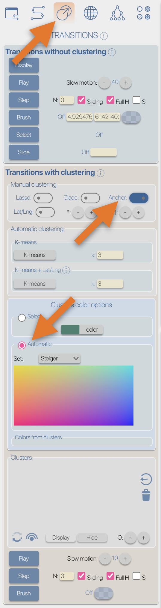
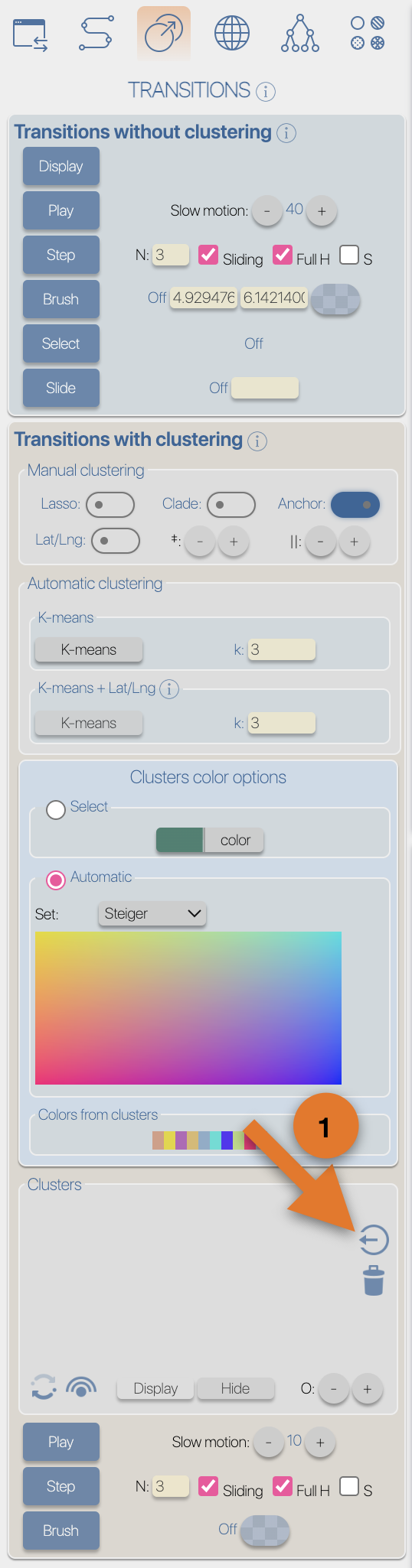
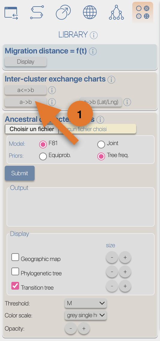
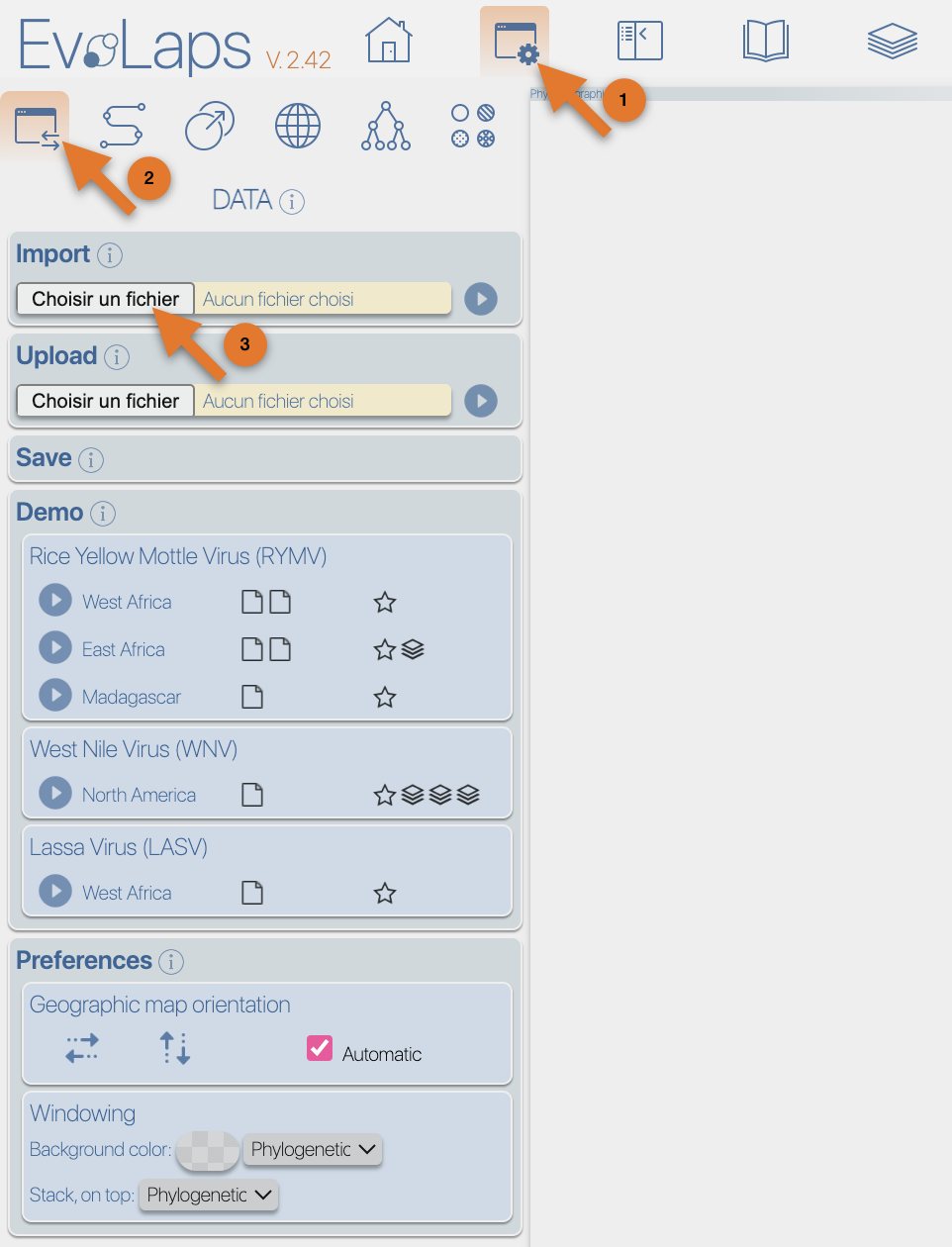
From the Top toolbox, select the "Process" button (1), select the 'DATA' toolbox (2), click the 'select file' button from the 'import' section (3), select the input file then click the 'submit' button.
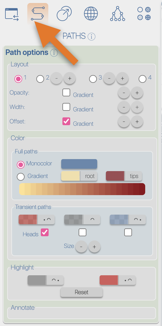
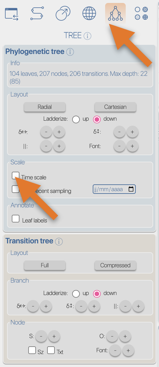
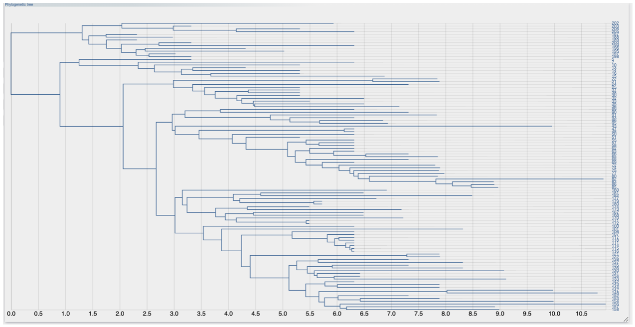
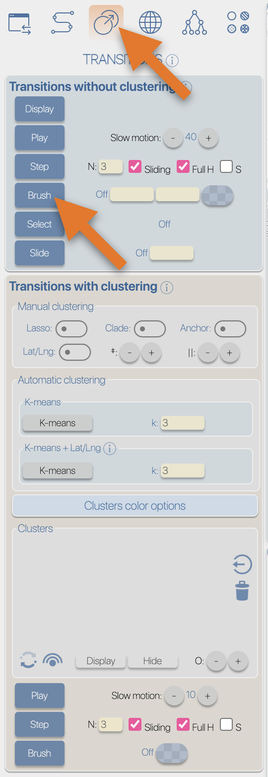
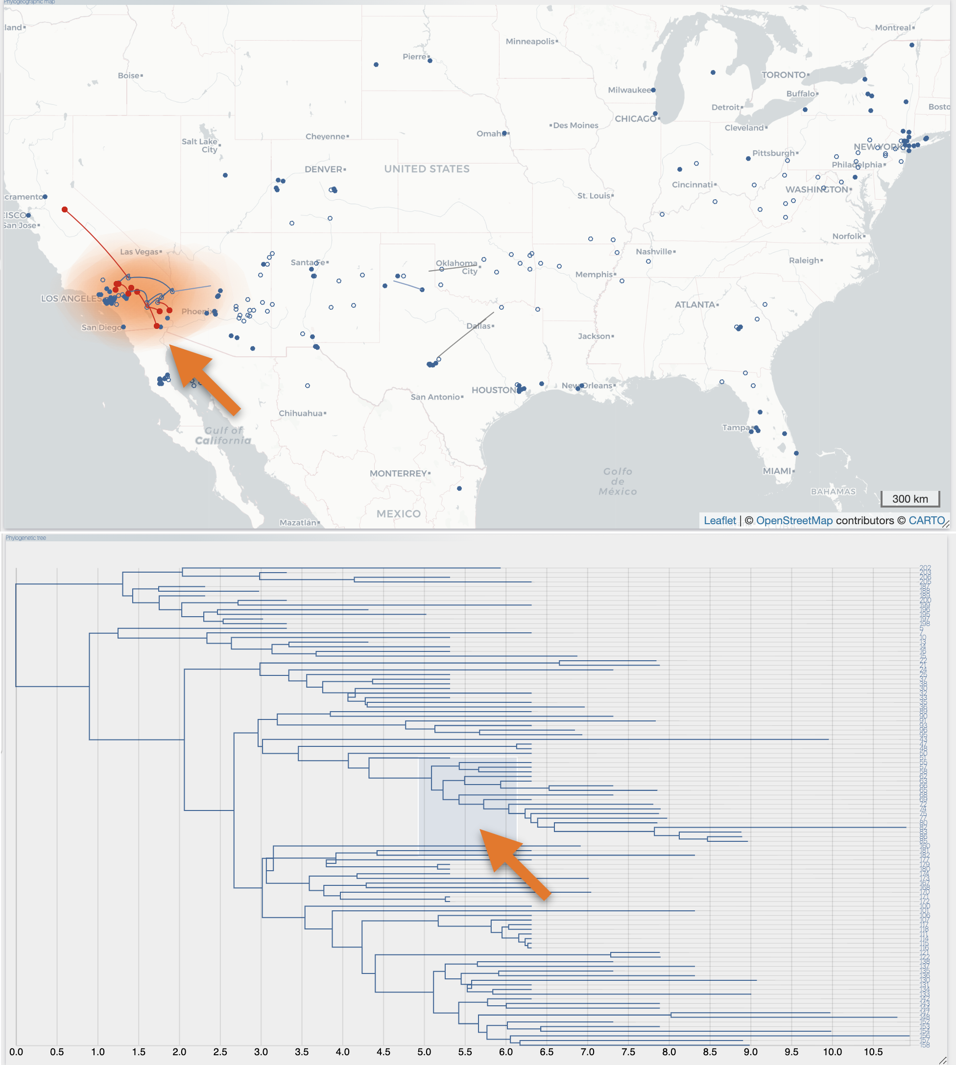
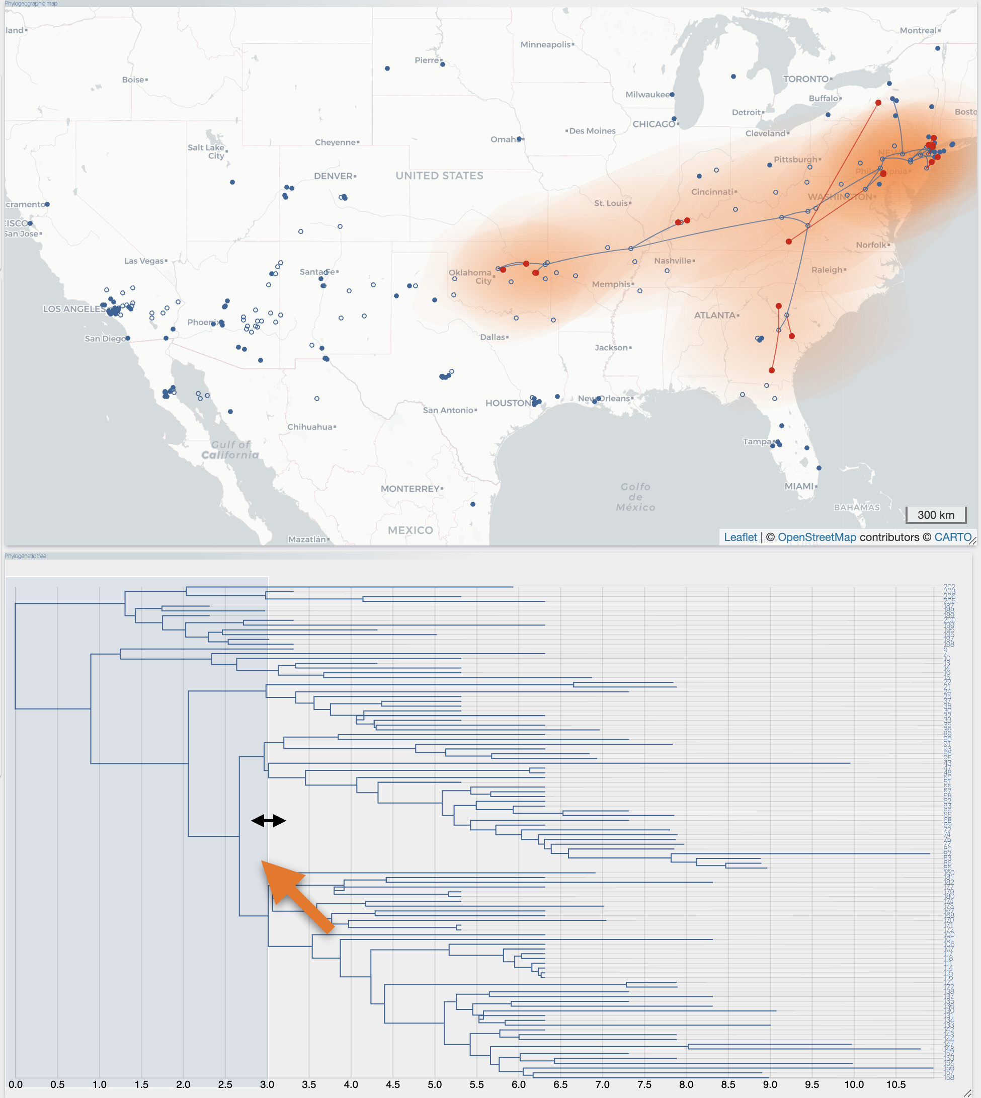
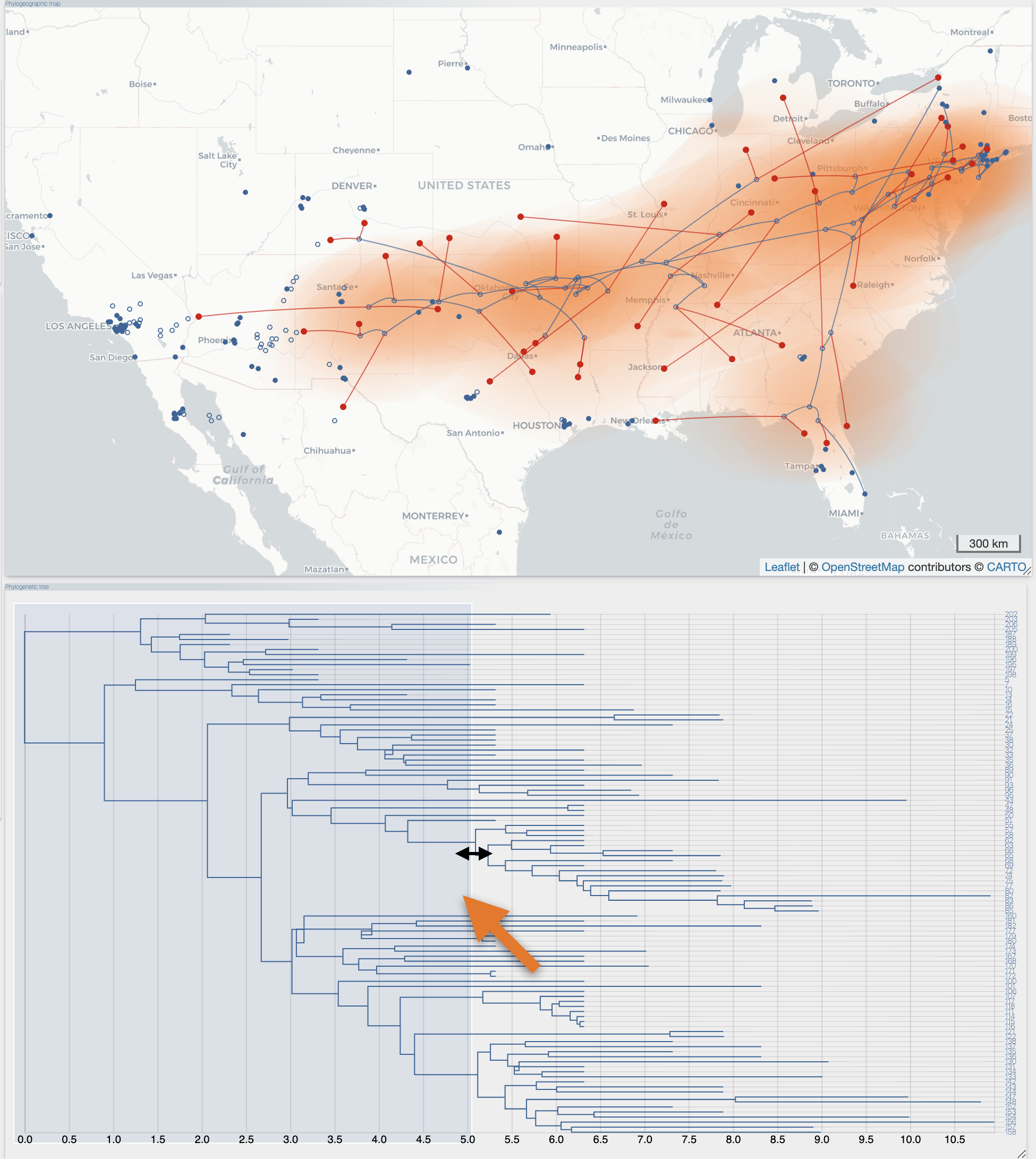
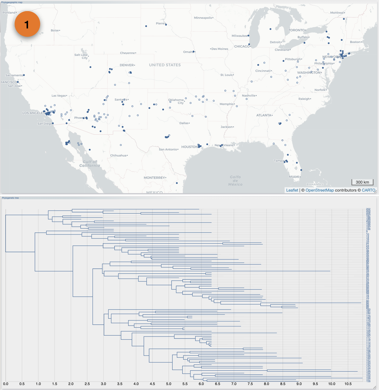
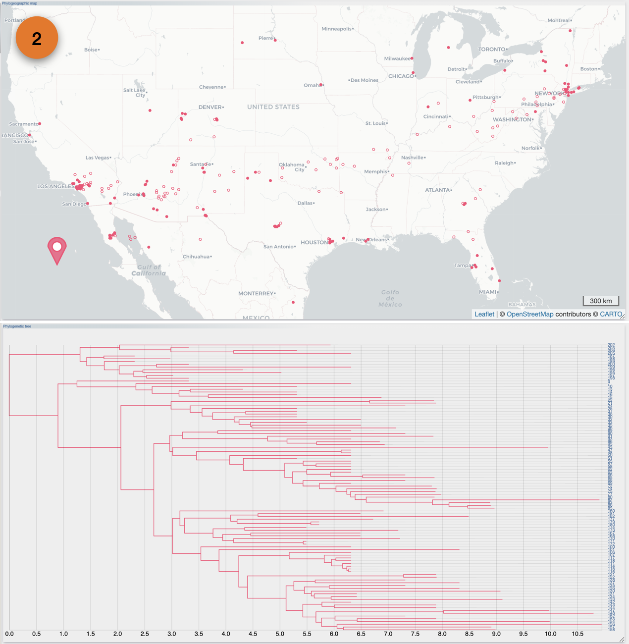
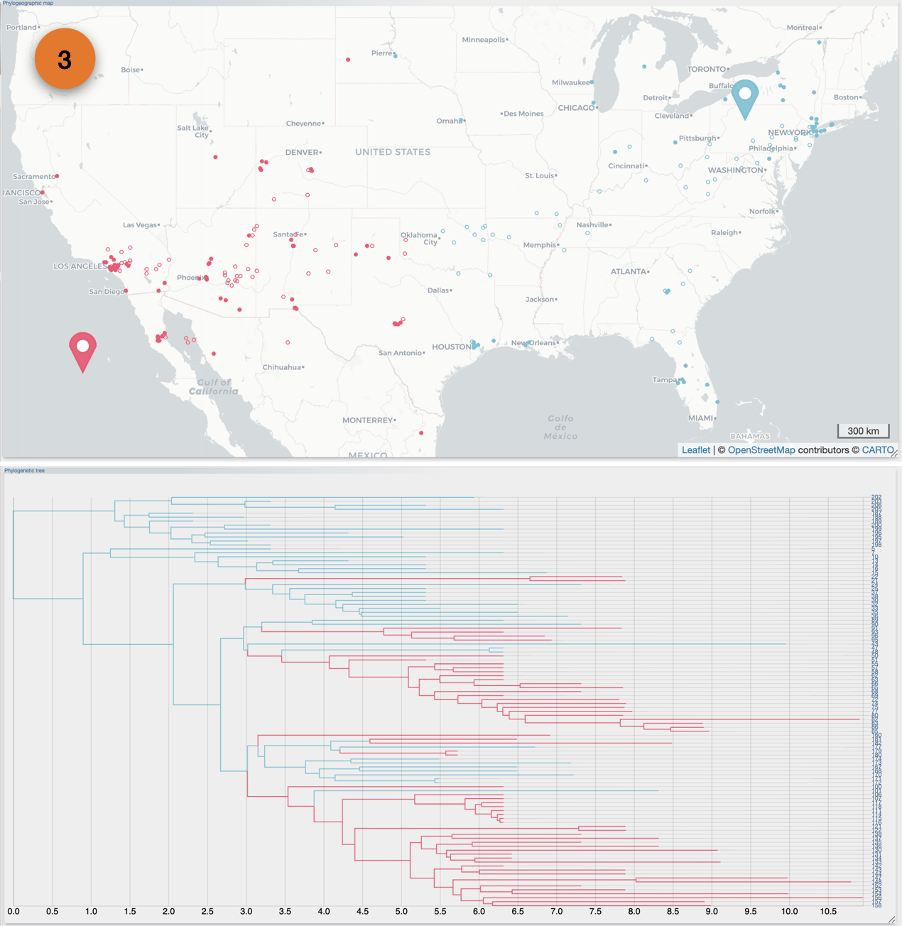
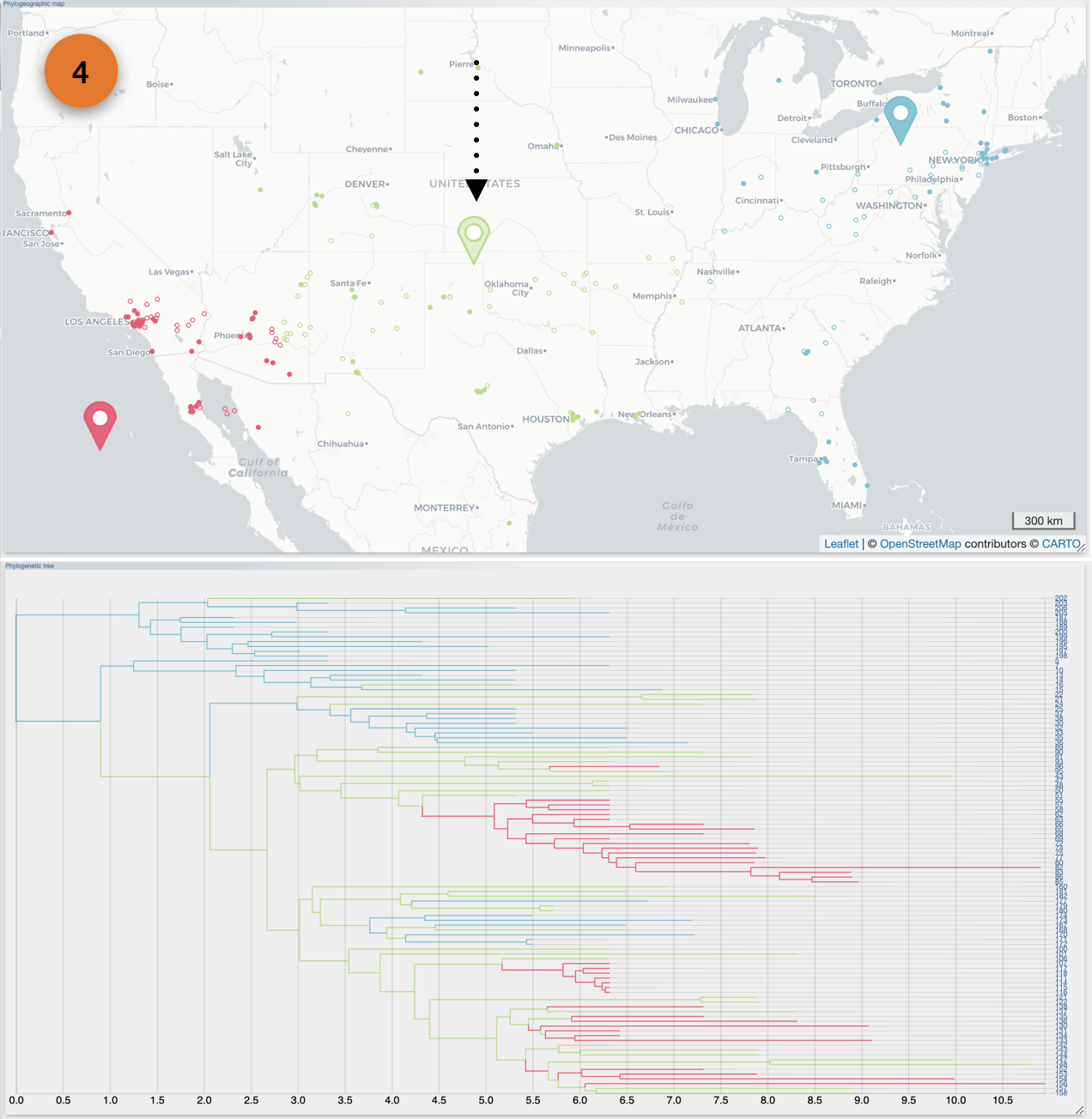
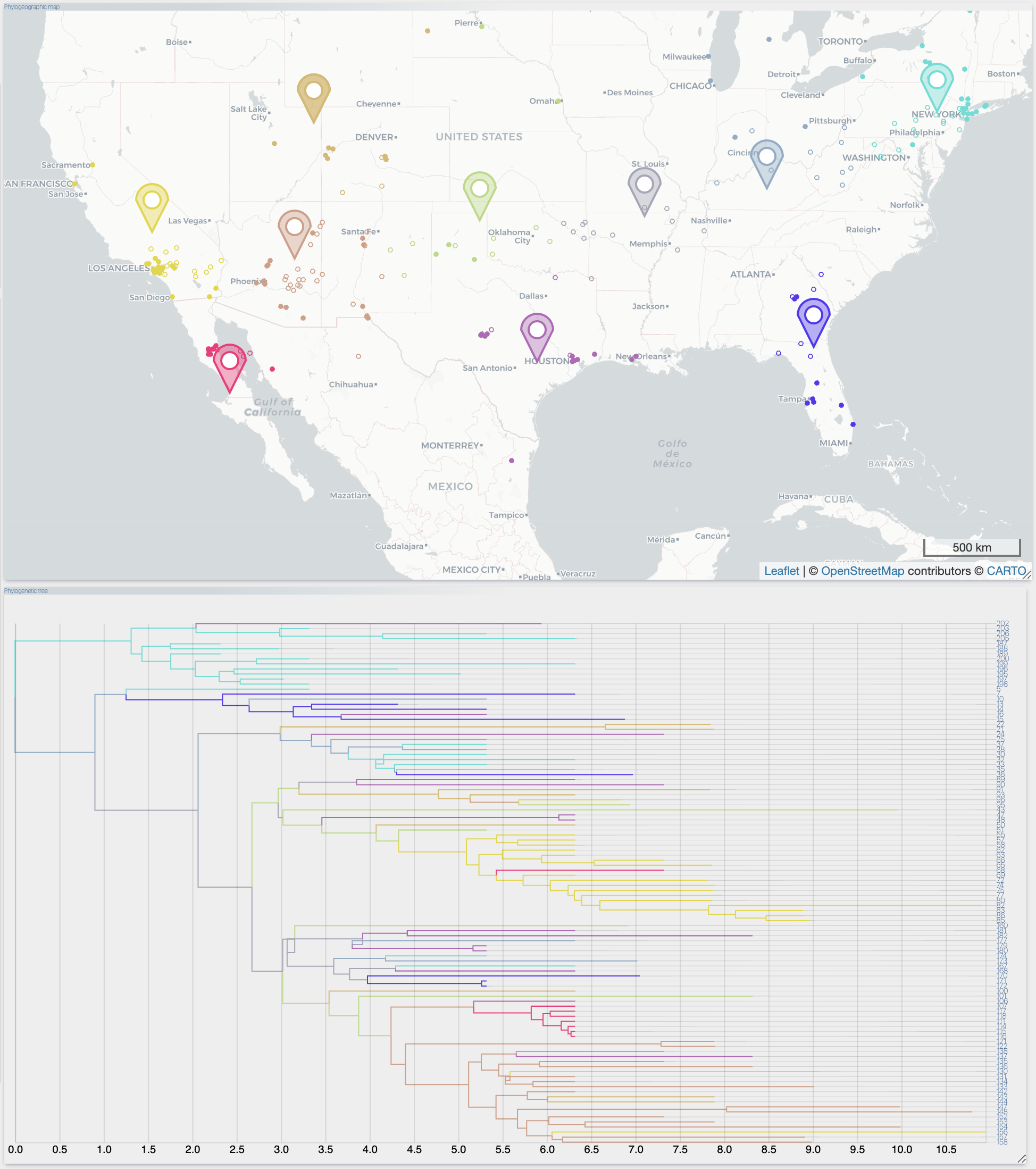
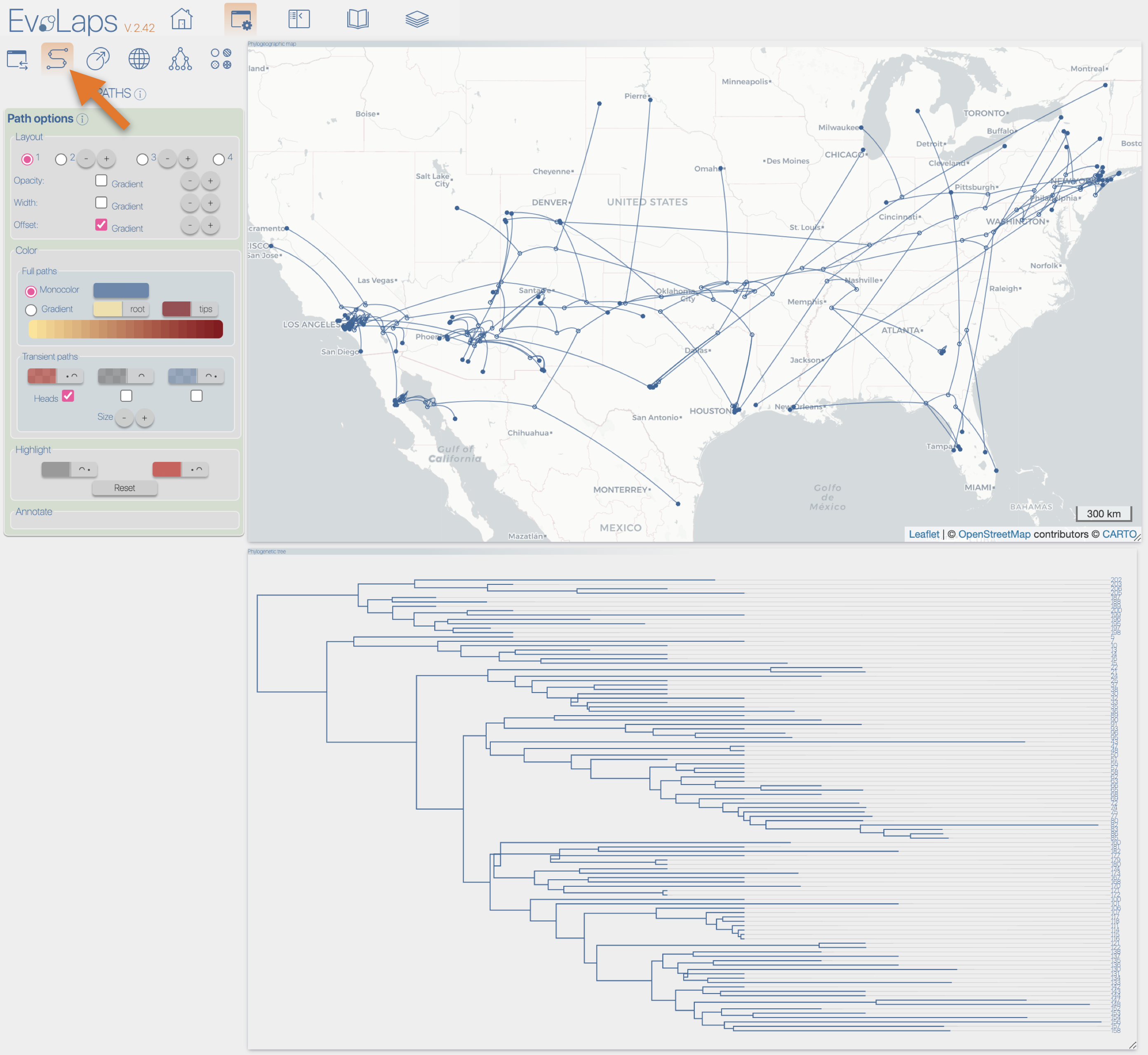
After the importation process, EvoLaps switch automatically to the 'PATHS' toolbox, and displays the geographic map with the phylogeographic scenario and the phylogenetic tree.

Layout of the phylogeographic scenario

The default layout of phylogeographic scenario is tuned from the 'Paths options'/'Layout' sections. Especially, it may be interesting to increase the depth of short migration distances
To add depth to the scenario :
  • uncheck the 'offset gradient' (1)
  • increase the offset by clicking the '+' button (2)
  • select the layout mode '2' (3)
  • click the '+' button of the mode '2' to increase depth of short distance migrations (4)

Displaying uncertainty zones associated with the most probable localities (HPD)

Depending of the analysis, HPD may be available, and with different treshold levels.
From the 'MAP' toolbox, opent hte 'Metadata' section and check on 'HPD'
Select a threshold (eg 80%)
Select a radial color gradient (two colors from the center to the boundaries, each with an alpha chanel)

Time and space decomposition of the spread

To provide a visualization of the successive stages of the dispersal in both time and space, the selection brush is used
Add a time scale to the phylogenetic tree
From the 'TREE' toolbox, 'Phylogenetic tree' section, check on the 'Time scale' control
Activate the selection brush
  • From the the 'TRANSITIONS' toolbox, section 'transitions without clustering', click the 'Brush' button
  • A default brush is displayed at the center of the phylohgenetic tree display
  • the phylogeographic scenario is restricted to this selection
Drag, move and resize the brush
  • the brush is moved to the root (t=0), resized to fit the full height of the phylogenetic tree with a width of 3 time units
  • a screenshot is copy/paste to a slideshow software
  • the brush is then resized again to fit t=5, and a new screenshot is copy/paste
NB 1 : check the FAQ section to learn how to obtain high-quality images
NB 2 : check the 'How-to' section 'Animation, brushing and partial paths'for having details on partial paths

Spatial areas definition

From the 'TRANSITIONS' toolbox, 'transitions with clustering' section, activate the 'Anchor' clustering method. The geographic map and the phylogenetic tree are reset (1).
Open the 'Clusters color options' tab, check on the automatic color setting and select a 2D matrix color, here the 'Steiger' palette is selected
Click the geographic map to create a 'red' anchor (2). The color of the anchor correspond to its relative position from the 2D color matrix. The nearest ancestral and sampled localities to the anchor are colored with the anchor's hue, indicating their cluster membership. The phylogenetic color is updated.
Click the geographic map to create a 'blue' anchor (3). The localities and the phylogenetic tree colors are updated.
Click the geographic map to create a 'green' anchor (4). Then move the anchor to the center of the map. Moving an anchor do not change its color. An anchor can be deleted with a right click on it. Again, the localities and the phylogenetic tree colors are updated
Move the desired number of dynamic anchors/clusters on the geographic map and, when satisfied, prompt the display of the corresponding phylogeographic scenario by clicking the button (1). Clusters are then represented as minimum convex hull polygons, with fill color specified by their original anchor.
The cluster list is automatically named (here 'clustering-0'). Each time you click this name (2) the corresponding scenario is displayed on the geographic map.
A transition tree is computed for each clustering (3). Revisiting the phylogenetic tree and assigning continuous localities to spatial clusters yields an inter-cluster transition tree. Projecting these inter-cluster transitions onto the geographic map allows for a simplified version of the phylogenetic scenario. The degree of simplification depends on the number of clusters. For more details related to the transition tree, see the 'Interface' and 'Transition tree' sections.

Transition chart

The transition chart provides inter-cluster exchange maps, which are matrix representations that cross-reference clusters and count the number of transitions between each pair of clusters.
click the 'a->b' button from the 'LIBRARY' toolbox (1)
Clusters, with their specific colors, are displayed using squares along the diagonal of the inter-cluster transition matrix. Numbers in the center of these squares are counts of intra-cluster transitions. Inter clusters transitions are represented by circles of a color specific to the donor cluster. Numbers in the center of these circles are counts of transitions from this cluster to the cluster in the same row, along the diagonal.
Here, the pointed grey cluster (2) has 5 transitions to the green clusters, which has in returns 2 transitions.
Pointing to a circle in the transition matrix dynamically highlights on the geographical map (3), both the donor and recipient clusters and displays an arrow pointing from the source to the target clusters.

Full tutorial in video