1. Introduction - LASV in West Africa - Tutorial 1

"... Lassa virus (LASV; Mammarenavirus lassaense) is a zoonotic arenavirus that causes a viral haemorrhagic illness in humans known as Lassa fever (LF). This disease has been recognized since the 1950s, and the virus was first identified in 1969 in the village of Lassa, Nigeria. Since its discovery, regular LF outbreaks have occurred in Benin, Guinea, Liberia, Sierra Leone, and Nigeria. An estimated 897,700 people are yearly infected by LASV, with 18,000 deaths occurring in the West Africa region..." (Bangura et al, 2024)

  • This tutorial is a step-by-step analysis. ***
  • Publication : Bangura, U., Davis, C., Lamin, J., Bangura, J., Soropogui, B., Davison, A. J., … Fichet-Calvet, E. (2024). Spatio-temporal spread of Lassa virus and a new rodent host in the Mano River Union area, West Africa. Emerging Microbes & Infections, 13(1)
  • PDF : https://doi.org/10.1080/22221751.2023.2290834
  • DATA: NEXUS file

Images and videos of this tutorial can be enlarged by clicking on them

2. Quick overview of the EvoLaps interface

EvoLaps is based on 5 windows:
  1. the Controls window: it contains 5 toolboxes for the phylogeographic analysis 1:
    DATAsubmit data: demo, import
    SCENARIOSscenario layout, style, animation, locations, clustering
    MAPgeographic map, hypsometric layer, environmental data layers
    TREEphylogenetic tree edition
    DOCUMENTATIONuser's manual
  2. the Map window: displays the phylogeographic scenario with geographic map and environmental data in the background. To navigate the map / the phylogeographic scenario:
    • move: the map by clicking it and dragging it
    • zoom: in and out using the mouse scroll wheel or two fingers on a trackpad
    • tilt and rotate: the map (or pitching and bearing of the camera) by clicking and dragging it while holding Shift (or right mouse button)
  3. Tree: displays the phylogenetic tree
  4. Library: a third-party display window for elements such as migration distance curves, transition graphs, etc
  5. Documentation: the user's manual
  • all windows are movable via drag-and-drop on their top frame (the mouse icon turns into a crosshair cursor)
  • the Map, Tree, Library, and Manual windows can be:
    • resized using their bottom-right corner
    • hidden by double-clicking on their top frame
    • 2 hidden or displayed through the controls in the DATA/Preferences section
  • the Tree and Library windows can either be embedded within the Map window (default option) or 3 detached (DATA / Preferences / In-Out mode)
  • the Controls panel always remains in the foreground, its background foreground colors, transparency, and font size can be customized 4
  • the Manual window can either be embedded in or detached from the main EvoLaps interface

For more details about the windows of EvoLaps, refer to the Interface > Windowing system section

Documentation window:

  • 1 Home of the documentation
  • 2 Toggle display of the documentation window (when it is not detached from the main EvoLaps window)
  • 3 Toggle detachment of the documentation window from the main EvoLaps window
  • 4 Adjust the font size of the documentation

The controls window

Navigation on the map window

3. Load the 'Lassa Virus (LASV)' data set

  • The 'Lassa Virus (LASV)' data set is available as a demo in EvoLaps. To launch the analysis with this dataset, go to DATA > Demo > Lassa Virus (LASV) & West Africa and click the Submit button 1.
  • click the star button if you want to save/edit the data 2

To submit data to EvoLaps, select a Maximum Clade Credibility Tree (MCCT) from the DATA > Import section button and click the submit button 3

If the analysis is based on a discrete model a Location file must be specified 4

After the importation step, EvoLaps switch automatically to the 'SCENARIOS' toolbox, and displays the phylogenetic tree, the geographic map with the phylogeographic scenario. Feel free to reflow the interface elements as needed

For more details about data format, refer to the File formats section

4. Geographic map settings

From the MAP toolbox:

  • 1 set the land color to white
  • 2 to reduce the relief rendering, set its hillshadow and hillhighlight colors to grey and light grey respectively
  • 3 check on the administrative countries border, and set its color to black
  • 4 check on the countries labels, set its color to black
  • 5 check on the settlements minor & major labels, set its color to grey

MapBox and OpenStreetMap acknowledgement EvoLaps maps are based on MapBox and OpenStreetMap. To display the copyright of MapBox and OpenStreetMap on the map, see DATA toolbox, preferences section. You can also add the figure comment with the following statement: "Prints use map data from Mapbox and OpenStreetMap and their data sources. To learn more, visit https://www.mapbox.com/about/maps/ and http://www.openstreetmap.org/copyright"

5. Layout & style of the scenario

1 
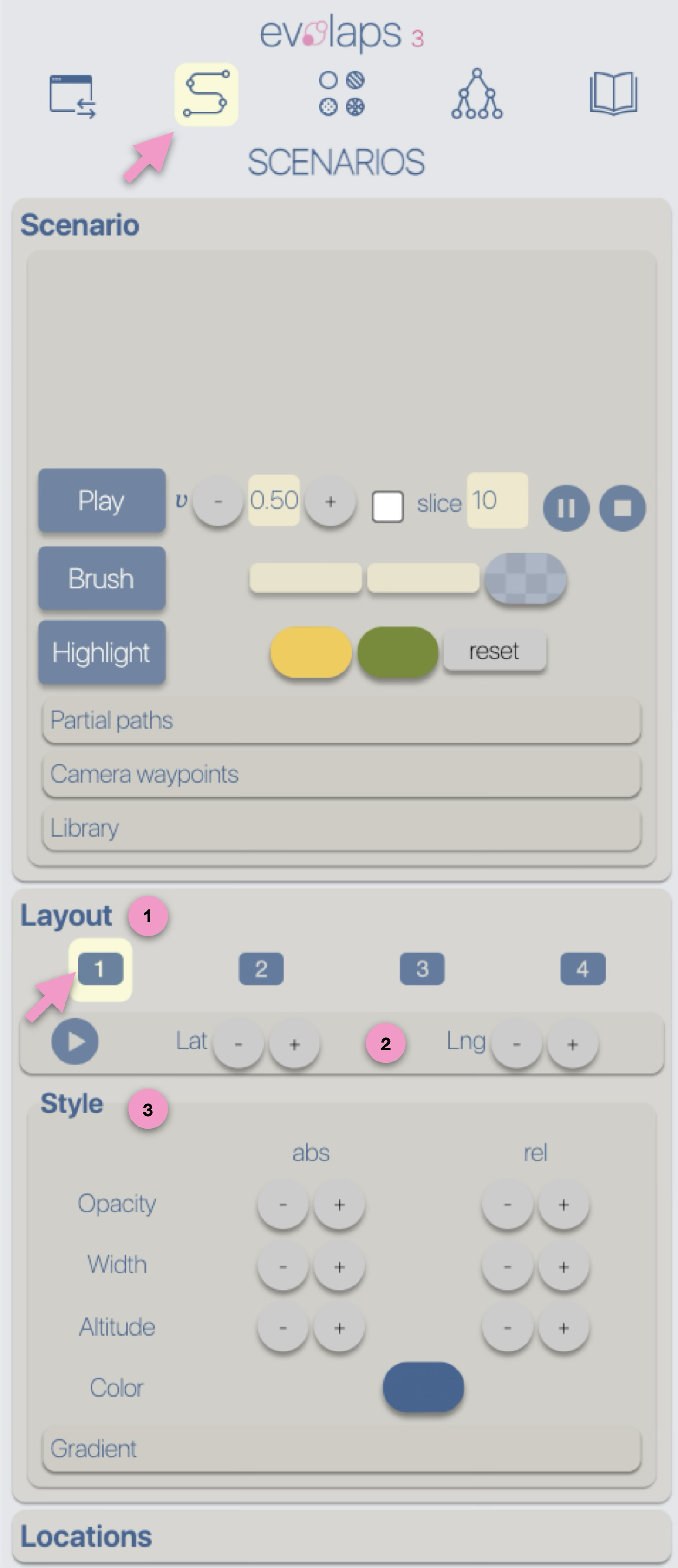
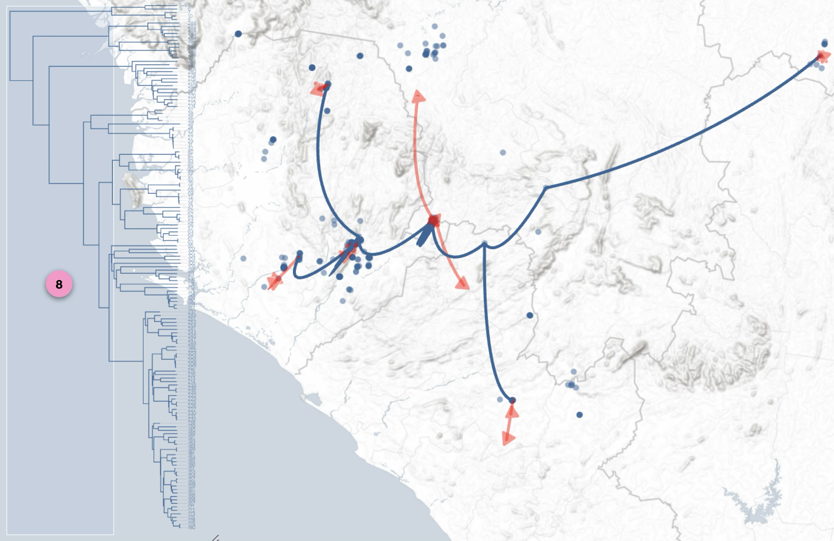
The graphical representations of phylogeographic scenarios (layouts) are grouped into families (currently four), based on the methods used to compute a path connecting points (latitude/longitude) associated with nodes of the phylogenetic tree (a parent node to its child nodes). For example, and without going into too much technical detail, layout family 1 implements a Bézier curve smoothing technique using three control points:

  • a first point (latitude/longitude) associated with a parent node,
  • a second point (latitude/longitude) associated with a child node,
  • an intermediate point calculated as the average of the latitude and longitude of the two previous points.

for more details related to the layout families, see the Phylogeographic scenario > Layout section.
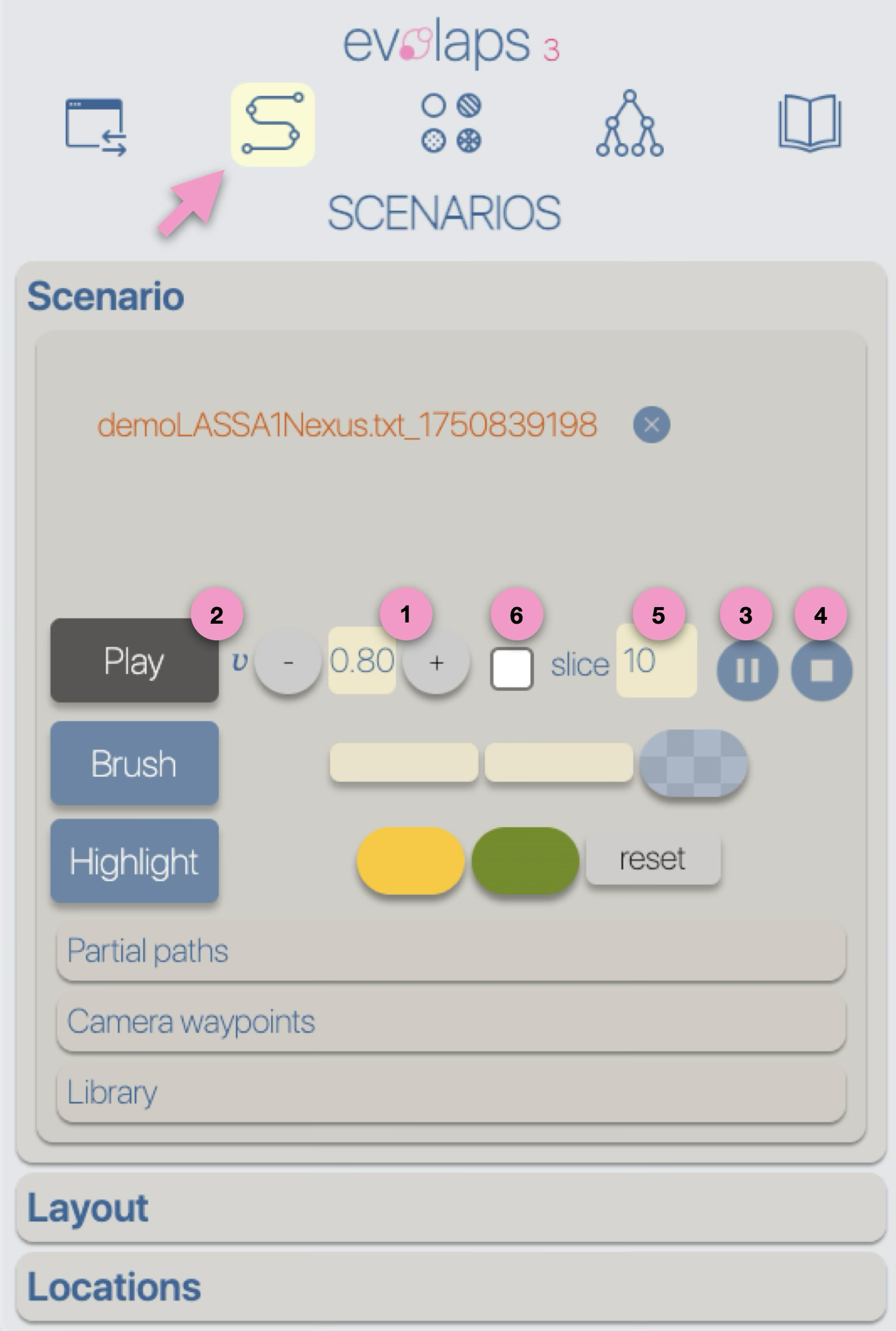
2 
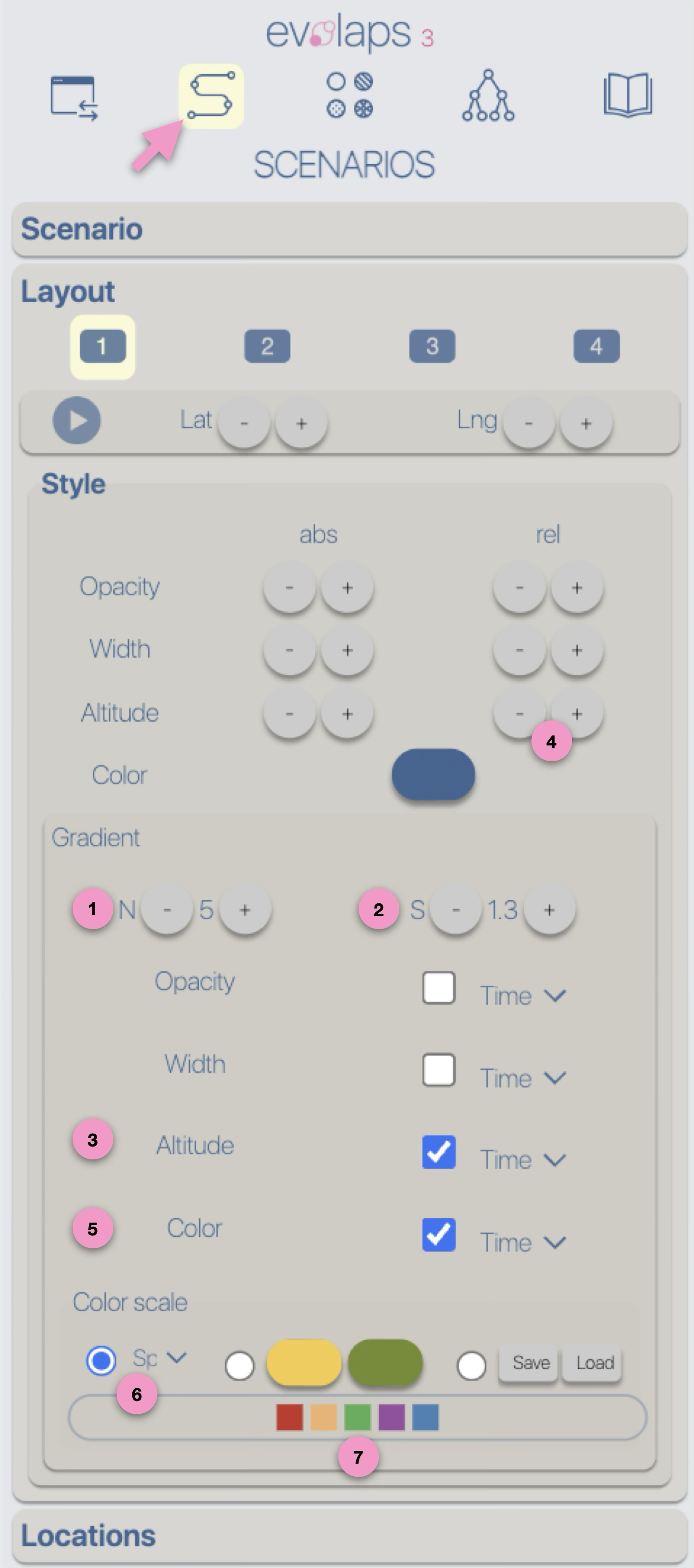
Layout-family-specific parameters allow for visual variations of the phylogeographic scenarios. For instance, family 1, provides an offset control for the latitude and longitude of the intermediate point.

Nota Bene: the graphical rendering quality of a phylogeographic scenario varies depending on the nature of the dataset, the different families/methods used to compute the paths may be more or less suitable.
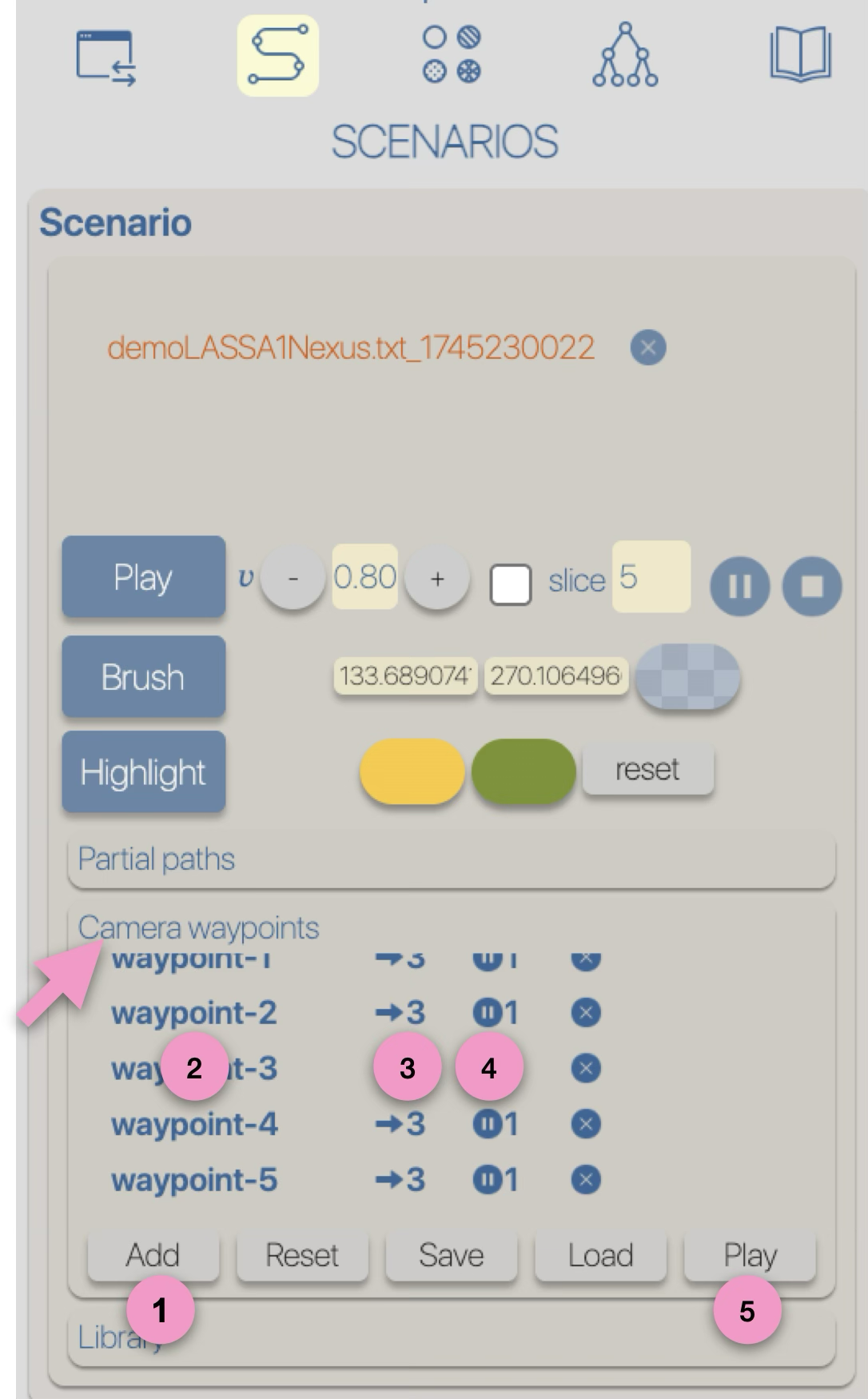
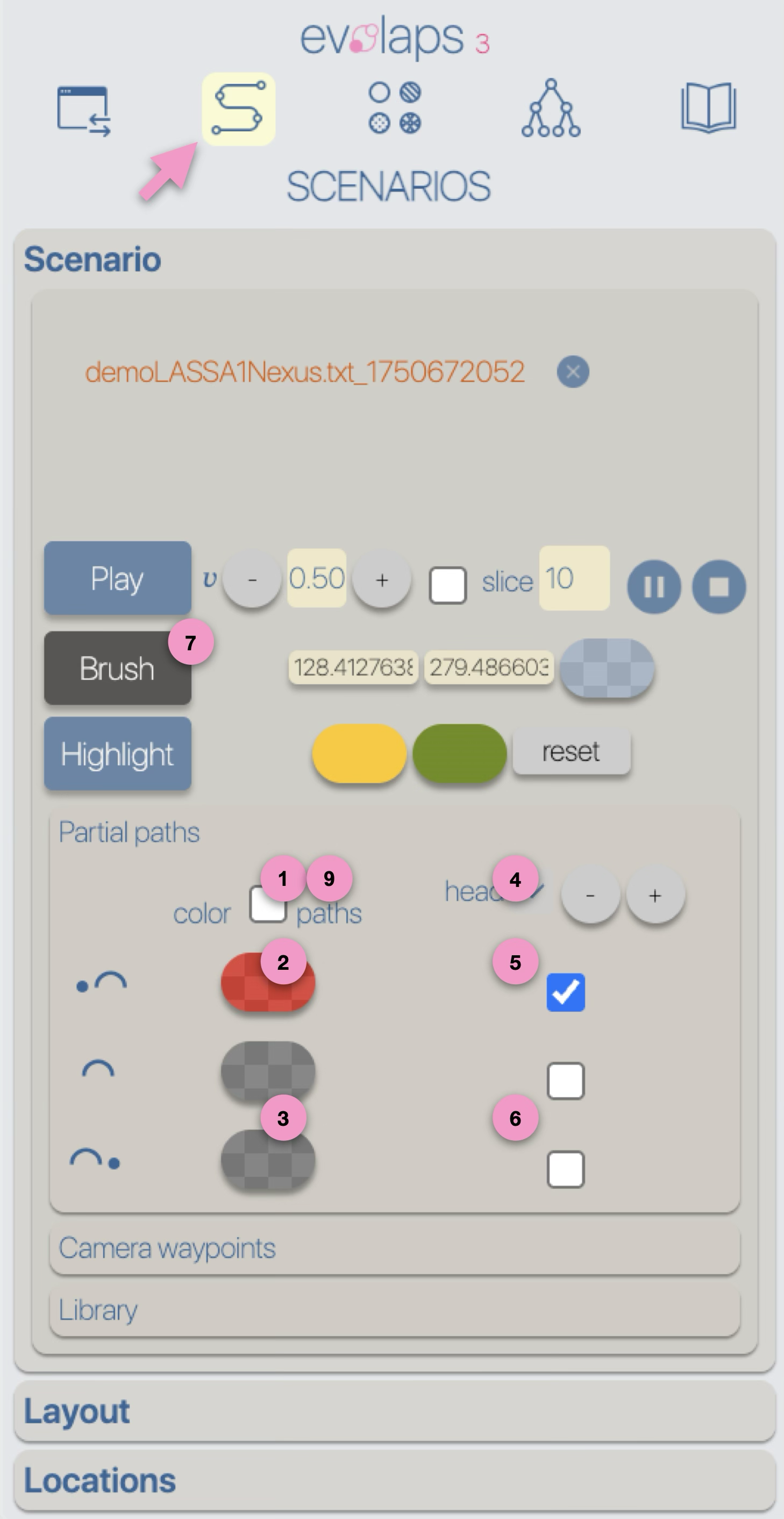
3 Style Regardless of the layout used to represent the phylogeographic scenario, it can be modified using four graphical variables: opacity, stroke thickness, altitude (curvature), and color. Apart from color, modifications (increase/decrease) can be either absolute ('abs'): the same value is applied to all paths in the scenario, or relative ('rel'): the existing value of each path is incremented (or decremented) individually. These modifications can be performed manually (using -/+ buttons) or automatically by applying a gradient (next step of the tutorial).

for more details related to the style, see the Phylogeographic scenario > Style section.

6. Add a time gradient (altitude, paths colors)

Opacity, stroke thickness, altitude (curvature), and color can be linked with a gradient. A gradient is configurable:

  • N is the number of classes
  • S is a stringency parameter between classes — the higher the S value, the stronger the contrast between classes

A gradient can be associated with:

  • Time: cumulative branch length from the node to the root of the phylogenetic tree
  • Distance: cumulative sum of geographical distances along the path from the node to the tree root. The distances are orthodromic (e.g., great-circle distances based on latitude and longitude between two points on a sphere)
  • Speed: Distance/Time ratio from the previous gradients

The color gradient has three options:

  • using a color scale. The colors in a scale are optimized, and the choice of scales is restricted depending on the number of gradient classes
  • selecting a start and end color
  • saving/loading a list of specific colors. The colors must be in hexadecimal format without transparency, listed in square brackets, for example: ["#d53e4f", "#fc8d59", "#fee08b", "#b5e61d", "#22b14b", "#a349a4", "#3288bd"]. In this example, the gradient can use up to 7 classes. The colors will be used in the order they appear in the list.

The color gradient classes (associated with time, distance, or speed) are represented by a list of colored boxes. Clicking on a box allows you to change the color of the corresponding class. Assigning the same color to multiple adjacent classes enables a non-linear color gradient. It is possible to use multiple gradients simultaneously — for example, a stroke thickness gradient based on time and a color gradient based on distance. Color gradients can be reflected on HPDs (see below the 'Displaying locations and HPDs' section) and on the phylogenetic tree (see below the 'Scenario & tree cross-selections' section).

  • From the SCENARIO toolbox:
  • 1 Set the number of gradient classes to 5
  • 2 Set the stringency to 1.3
  • 3 check on Altitude and link it to a time gradient
  • 4 lower the relative altitude to clearly distinguish the five time classes and visualize the scenario as a bouncing ball
  • 5 check on Color and link it to a time gradient
  • 6 Select the 'Spectral' color scale
  • 7 Click the color boxes to switch the yellow and light green colors to green and purple

7. Displaying locations and HPD

EvoLaps allows separate display of sample and ancestral locations, using filled or empty circles, with customizable size and color.

  • From the SCENARIO toolbox / Locations section :
  • 1 check on the sample and ancestral locations display
  • 2 check off the full circle for ancestral locations
  • 3 select a red color for ancestral locations and a green color for sample locations
  • 4 check on the display of HPD at 80%
  • 5 check on/off the path color option

8. Scenario animation: 'Brush'

The phylogeographic scenario animation is based on a phylogenetic tree brushing process.

In the Brush mode, a default brush is displayed at the center of the phylohgenetic tree display with a default size. The phylogeographic scenario is restricted to this selection. The size and position of the selection brush are variable, either determined by the user on-the-fly or automatically ('Play' mode, see below). The use of a selection brush enables the display of a phylogeographic scenario limited to a specific clade and/or time slice, with paths that may be partial.

Partials paths

  • on the geographic map, a path between two points is full when the corresponding nodes (parent and child nodes) are within the brush selection from the phylogenetic tree
  • the path is partial if none of the associated nodes are within the brush selection, which lies between the two nodes of the tree
  • if the parent node is within the selection but not the child node, the path is downstream partial
  • if the child node is within the selection but not the parent node, the path is upstream partial
Length of a partial path is proportional to the branch length included in the selection. Partial paths can be distinguished with different graphical characteristics, such as heads and/or color. Partial paths can also adopt the color of their full paths, meaning they can follow a gradient or clustering scheme.

From the SCENARIO toolbox / Scenario section:
  • 1 uncheck the path color option
  • 2 select a red color for downstream partial paths
  • 3 select a grey color for partial paths and upstream partial paths
  • 4 select 'arrow' for heads
  • 5 check on the head option for downstream partial paths
  • 6 check off the head option for partial paths and upstream partial paths
  • 7 click the 'Brush' button
  • 8 on the phylogentic tree move/resize the brush
  • 9 now, check on the path color option and move/resize the brush to see the time color gradient (step 6 of the tutorial) for all the partial paths

(video)

9. Scenario animation: 'Play'

The ‘Play’ mode has two functions: a normal mode (default) and an optional slice mode.

In normal mode, the brush remains in the same position, but its width increases over time. In slice mode, the brush moves over time (translation), but its width remains constant.

This width is adjustable as a percentage of the total phylogenetic tree duration (here 10%). Both modes include controls for pausing/resuming the animation and stopping it entirely. During a pause, graphical parameters of the scenario (HPD display, path colors, gradients, etc.) can be adjusted on the fly. Both modes respect the selected animation speed, controlled by parameter ‘v’ ranging from 0.1 (slowest) to 0.9 (fastest).

From the SCENARIO toolbox / Scenario section:
  • 1 set the speed to 0.8
  • 2 click 'Play'
  • 3 click the 'Pause' button to stop the animation, click it again to resume
  • 4 click 'Stop' to stop the animation
  • 5 set the 'Slice' value to 5% and check on the 'Slice' option
  • 6 click 'Play'

(video)

10. Scenario & tree cross-selections

Pointing to a node in the tree highlights its origin all the way to the root, as well as the underlying clade, using two user-selected colors: an ‘upstream’ color and a ‘downstream’ color, respectively. This process automatically reflects on the phylogeographic scenario: the ‘upstream’ color overlays the phylogeographic scenario from its starting point to the selected node, while the associated migration paths of the clade are highlighted with the ‘downstream’ color. Conversely, pointing to a path in the phylogeographic scenario allows highlighting the upstream and downstream areas of the phylogeographic scenario, as well as the corresponding branches within the phylogenetic tree. Selection is performed using the same method, but with a mouse click, allowing the user to preserve the highlighted areas. The ‘upstream’ and ‘downstream’ colors can vary (user’s settings) between different selections.

  • From the SCENARIO toolbox:
  • 1 click 'Highlight'
  • 2 navigate the tree or the scenario to highlight upstream/downstream paths (tree and scenario)
  • 3 click different paths (tree or scenario) to preserve the highlight with different downstream color selections
  • 4 click the 'Reset' button to clear the highlight

(video)

11. Add a migration distance curves

  • From the DATA toolbox:
  • 1 ...
  • 2 ...

(image)

(video)

12. Effective use of Lasso selections

EvoLaps incorporates a set of tools to group ancestral and sampled localities into spatial clusters. All ancestral and sampled locations do not necessarily have to belong to a cluster. For example, it is possible to define a single cluster using the Lasso tool to better visualize the incoming/outgoing paths of a given area.

To define a cluster using the Lasso tool, hold down the space key, then click on the map and draw the geographic area that includes the locations you want to cluster. The Lasso can also be used to split or merge existing clusters. Cluster colors can be assigned either manually or automatically.

When a cluster (or a list of clusters) is defined, the following operations are available:

  • From the SCENARIO toolbox:
  • 1
  • 2
  • 3
  • 4
(video)

13. Camera waypoints

Camera waypoints allow you to create smooth, animated transitions—ideal for producing animations to include as supplementary material in a publication.

  • From the SCENARIO toolbox:
  • 1 Open the 'Camera waypoints' section, initialize the map (zoom, tilt, etc), click the 'Add' button.
  • 2 clicking on a waypoint's name automatically navigates the map to that point
  • set a transition time to this waypoint (seconds)
  • 3 set a pause duration at this waypoint (seconds)
  • 4 click the 'play' button to preview the animation. The waypoints list can be saved and loaded.

14. Add a hypsometric layer

  • From the DATA toolbox:
  • 1 ...
  • 2 ...

(image)

(video)

15. Save the analysis

  • From the DATA toolbox:
  • 1 ...
  • 2 ...

(image)

(video)